2025-03-aes-twitter-logfav-transforms

The model training has been concluded;

See: https://huggingface.co/incantor/aes-twitter-cbrtxlog-siglip2-base

Intuition

Human feedback is limited. We want to collect aesthetic feedback efficiently, and at scale.

→ How can we make better use of social media feedback?

Twitter Data

Twitter data is inherently noisy:

From what I recall, the figures are roughly:

• About half of the posts are not artworks (~40%).
• Many are from amateurs (the mean like count is around 80).
• AI-generated images are widespread and unlabeled.
• We need to distinguish actual illustrations from rough sketches, gacha game screenshots, and various unrelated content.
• We also need to avoid including Nightshade-protected images.

This experiment focuses on the transformation side of the problem, leaving other challenges for later.

Transformations on Twitter

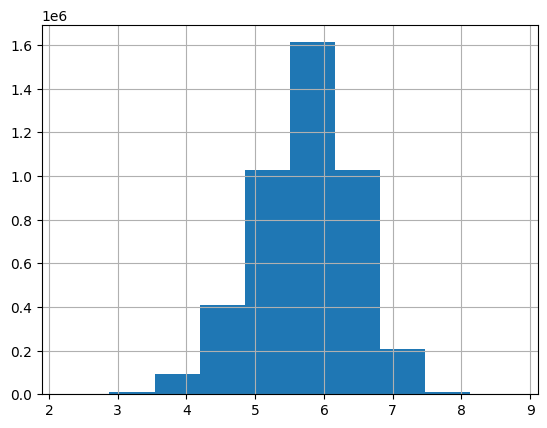
Twitter engagement data (like counts) tends to follow a normal distribution after a log transformation:

• (Also See: lark document)

Based on these characteristics:

1. Twitter likes follow an inverse log distribution.
2. We want to distinguish high-quality images from lower-quality ones.
3. The most informative range appears to be between 200 and 20k likes.

We propose three transformations:

# Define transformations
def transform1(x):
    # Converts the distribution to something close to bell-shaped
    return np.log1p(x)
 
def transform2(x):
    return np.sqrt(x) * np.log(x + 10)
 
def transform3(x):
    # Emphasizes the range between 200–20k likes, which empirically captures key distinctions in aesthetics
    # Still right-skewed; results in slower convergence and significantly higher loss (~10–20x compared to log1p)
    return np.power(x + 1, 1/3) * np.log(x + 10)

Discussion on Transformations

Better gradient behavior?

• log1p(x) provides a smooth, well-behaved gradient.
• In contrast, cbrt × log (transform3) involves a power transform and lacks a closed-form gradient, making optimization harder.

Better numerical range?

• cbrt × log was designed so that, under constant error in the transformed space, it minimizes absolute error in the range of 200 to 20k likes—an empirically important aesthetic band.
• We trained on both log1p and cbrt × log, and evaluated error across real value ranges (after projecting back).
• Finding: both transformations tend to underestimate the popularity of good artworks.

Better architecture?

• Trained with log1p on both DINOv2-Large and SigLIP2-Base. Compare differences in error profiles and convergence.

Better hyperparameters?

• In the DINOv2 experiment, slightly adjusted learning rate. Results suggest sensitivity—worth deeper inspection.

Transformation vs. loss penalties?

• A good transformation can simplify the optimization problem, possibly avoiding the need for custom loss penalties.
• However, some transformations—like cbrt × log—can distort the gradient too much, making convergence more difficult despite better range coverage.

Distribution mismatch?

• Predictors trained on full Twitter data tend to underestimate like counts for high-performing artworks.

We’re predicting Twitter favorite counts for artworks using either log1p(x) or transform3 (cbrt × log)—applied to the target or as a feature.
After training, predictions consistently fall below actual values. With more training (e.g., from 9k to 22k iterations), the total predicted likes decrease, despite loss continuing to improve.

Example:

# some sample labels on the same set
sum(predictions_9k), sum(predictions_22k) 
(258.18, 242.20)

This underprediction aligns with the underlying distribution:

• Twitter engagement is heavily skewed—most posts have low like counts (mean ~80).
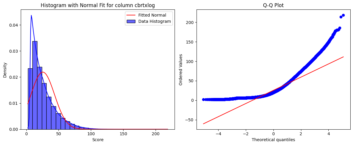
• After transformation, the target distribution becomes:

count 3,632,472 
mean 25.44 
std 18.20 
min 2.30 
25% 11.63 
50% 20.10 
75% 33.92 
max 218.70

Key insight:
MSE penalizes large errors more heavily.
So: when the transformation expands high-value ranges (e.g., cbrt × log), the model becomes more conservative—it minimizes loss by shrinking predictions near the dense low-like region.

Additional observations:

• Even after transformation, predictions remain too small compared to the original like counts.
• Longer training (more steps) often leads to lower predictions, not higher.

Model Outcomes

Two versions of the model using the cbrt × log transformation are available on Hugging Face:

incantor/aes-twitter-cbrtxlog-siglip2-base-s9600

• Early checkpoint (~9.6k steps)
• More uniform predictions, avoids overfitting to outliers
• Often preferred for evaluation due to stable performance
• Sample outputs show cleaner aesthetic curation

incantor/aes-twitter-cbrtxlog-siglip2-base

• Later checkpoint (~22k steps, 1 epoch)
• Trained on ~3.6M Twitter favorites
• Captures broader signals, but more sensitive to noisy high-like posts (e.g., memes)
• Produces slightly more diverse but less consistent scores

Notes:

• Trained with SigLIP2-base on cbrt × log transformed favorite counts to emphasize mid-range aesthetic signal (200–20k likes).
• Despite improved numerical targeting, the model tends to underpredict high-like posts—similar to log1p—due to MSE and skewed data.
• Longer training reduces predicted scores slightly (e.g., from 258 → 242 on a fixed sample), aligning with earlier loss trends.

# sample from eval:
sum(preds_9k), sum(preds_22k)
# → (258.18, 242.20)

Performance Snapshot:

Metric	Value
Eval RMSE	13.84
Eval MSE	191.52
Train Loss	221.35
Eval Samples	~72k

These values are relatively high—likely due to the expanded value range and more erratic gradients from the cbrt × log transformation.

Evaluation:

• Model is not state-of-the-art, but usable for aesthetic ranking with Twitter-style engagement.
• Produces visually coherent high-score outputs from 10k+ unseen images.
• Earlier checkpoint tends to filter better; later checkpoint captures more outliers.

---

Appendix: Error Visualization

Error Simulation (1): Global Range

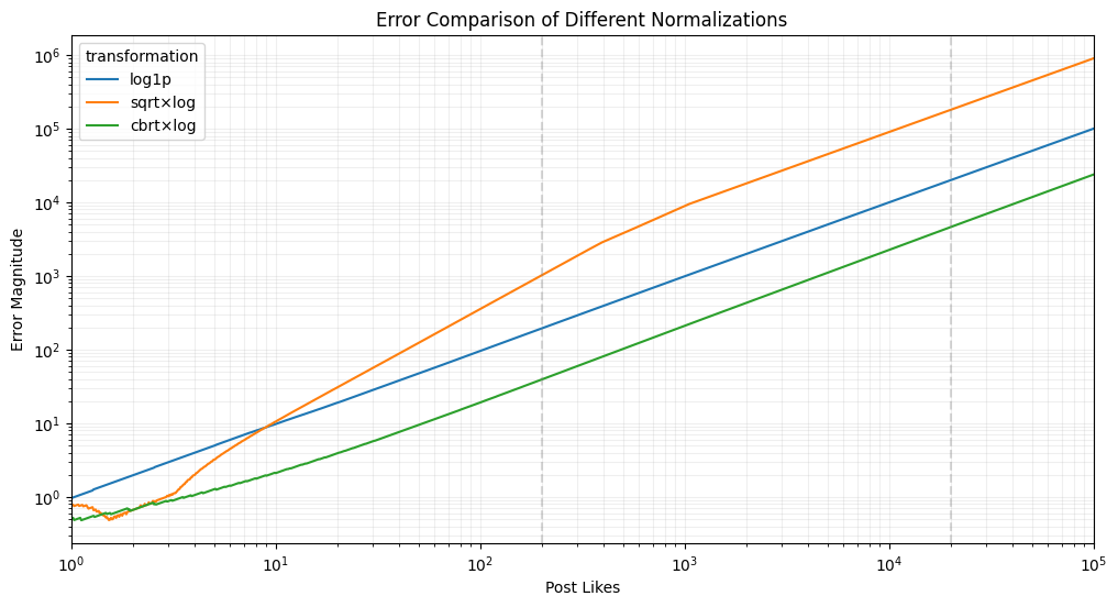
We simulated how a ±10% error in the transformed space maps back to original values for each transformation. Results were plotted over a wide range of post likes (1–100k).

Transformations:

def transform1(x): return np.log1p(x)  
def transform2(x): return np.sqrt(x) * np.log(x + 10)  
def transform3(x): return np.power(x + 1, 1/3) * np.log(x + 10)

The method used binary search to estimate inverse error in original space, assuming uniform relative error in the transformed space.

Outcome: cbrt × log has the lowest error in the upper range (20k+), but not always in the mid-range. The curve is less steep and better spaced for higher values.

---

Error Simulation (2): Focused Range (200–20k)

See full notebook: Error Analysis Comparison

To better understand the behavior in the range we care about most, we zoomed in on 200–20k likes, using the same method.

# Average errors in 200–20k range
{
    'log1p': 10982.25, 
    'sqrt × log': 1664.97, 
    'cbrt × log': 2299.06
}

Summary:

Transformation	Avg Error (200–20k)
log1p	10,982 (worst)
sqrt × log	1,665 (best)
cbrt × log	2,299 (middle)

Takeaways:

• sqrt × log performs best in the 200–20k range—the aesthetic sweet spot.
• cbrt × log offers a smoother curve and excels at higher values, but sacrifices mid-range precision.
• log1p significantly underperforms across the board.

This highlights a key tension: optimizing for aesthetics may require non-standard transformations that deviate from typical log-based scaling, even if they complicate gradient behavior.