2025-03-twitter-logfav-transforms

Eval ideas (on twitter logfav):

The goal is to train an aesthetic predictor (or: predict the like count receives by an artwork, given some twitter artowrks data):

there are few transforms to test:

# Define transformations
def transform1(x):
	# converts distribution to near-bell-shaped
    return np.log1p(x)
 
def transform2(x):
    return np.sqrt(x) * np.log(x + 10)
 
def transform3(x):
	# maximizes numeridcal range 200-20k, which is emprically found to be important distinctions of aesthetic; still heavily skewed right
	# also: had significantly slower convergence compared to log1p(and much higher loss, like 10-20x)
	# transform was there to make the model predict more precisely on value range 200-20k
    return np.power(x + 1, 1/3) * np.log(x + 10)

better gradient?

log1p(x + 10) : straightforward gradient, vs. current (a power transform, difficult grad)
cbrtxlog: do not have a close-formed solution.

beter numerical range?

cbrtxlog is designed so if error is constant, it gives less error from 200 to 20k.
train on both log1p and cbrtxlog, and see error difference across real value ranges (after projecting back)
finding: both log1p and cbrtxlog tend to underestimate good artworks.

better architecture?

train on log1p on both dinov2-large and siglip2-base

better hyperparameters?

On dino v2 experiment, changed LR a bit; analyze results

transformation vs. loss penalty?

if transformation fixes it, it could be more straightforward (compared to hacking loss)
some transformations may make optimization harder by messing with gradient /derivatives too much: (eg. cbrt x log compared to just stable log1p)

distribution mismatch?

predictor trained on full twitter gives lower values of like count compared to actual data

You’re predicting Twitter favorites count (target) for artworks, using either log1p(x) = np.log(x + 1) or transform3(x) = np.power(x + 1, 1/3) * np.log(x + 10) as transformations—either on the target or as features. After training, your predictor consistently underestimates the true favorites count, and with more training (e.g., from 9k to 22k iterations), the predictions drop further (sum of predictions: 258.18 → 242.20 on some sample set), even though loss/MSE keeps decreasing. You suspect the population’s mostly low likes are to blame.

(after cbrtxlog transform); original mean was around 80 likes

count    3.632472e+06
mean     2.544201e+01
std      1.819762e+01
min      2.302585e+00
25%      1.162599e+01
50%      2.010249e+01
75%      3.392451e+01
max      2.186985e+02

AND: MSE loss minimizes large errors. so: by increasing value range (cbrtxlog, it’s being more conservative to higher values).

observations:

After using transform the predictor still tends to predict a much smaller value of likes compared to original?
also by continuously training the model, the prediction goes lower:

# some sample labels on same set
sum(labels_9k), sum(labels_22k)
(258.1785879135132, 242.20263767242432)

Key Points

Use

\sqrt{\text{post\_likes}} \times \log(\text{post\_likes} + 10)

for better predictions in the 200-20,000 like range.
This transformation gives a larger spread in the transformed space, helping the model distinguish better.
Normalize transformed data for model training to handle non-normal distributions.

Why This Transformation?

The goal is to train a regressor to predict X like counts, focusing on the 200-20,000 range, where the current log1p(like_count) compresses higher values, making the model less sensitive. The proposed transformation,

\sqrt{\text{post\_likes}} \times \log(\text{post\_likes} + 10)

, stretches this range, giving the model more room to learn differences.

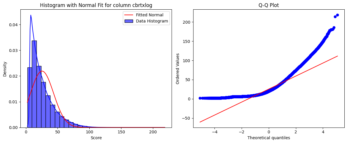
Error Distribution and Normality Trade-off

For the 200-20,000 range, errors are lowest with

\sqrt{\text{post\_likes}} \times \log(\text{post\_likes} + 10)

at 1,664.97, compared to 10,982.28 for log1p and 2,299.06 for the cube root version.
However, log1p achieves the most normal-like shape, followed by the cube root, then the square root version, which might affect model training for some algorithms.

Surprising Detail: Multiplication Enhances Sensitivity

Multiplying

\sqrt{\text{post\_likes}}

\log(\text{post\_likes} + 10)

creates a larger spread (1,325.64 units) in the 200-20,000 range compared to log1p (4.6 units), improving model focus without overwhelming with outliers.

Survey Note: Detailed Analysis of Transformations for X Like Counts in Regression

This section provides a comprehensive analysis of handling skewed and imbalanced X like counts for illustrations, focusing on transformation techniques to emphasize the 200-20,000 like range for regression tasks. The goal is to address the user’s need for a transformation that enhances model performance in this range while considering the trade-off with normality, which might affect model training.

Background and Problem Context

X like counts for illustrations often follow a power law distribution, with most X posts receiving few likes (e.g., 0) and a few receiving extremely high counts (up to 200,000). This skewness poses challenges for regression models, particularly when the user wants the model to be more sensitive to the mid-to-high range (200-20,000 likes) rather than the lower end (near 0), which is often filtered out. The current approach of using log1p(like_count) (i.e., log(1 + like_count)) compresses higher values, making the model less responsive to differences in the desired range, leading to poorer performance as like counts increase.

Transformation Techniques for Skewed Data

To address this, we explored common transformations for skewed data, drawing from machine learning literature. Standard methods include:

Logarithmic Transformations: log1p(x) is popular for handling zeros and compressing right-skewed data, but it flattens higher values, reducing sensitivity (e.g., the difference between 20,000 and 200 likes is only 4.6 in the transformed space, per calculations).
Power Transformations: Square root (sqrt(x)) or cube root (x^(1/3)) reduce skewness, suitable for count data, but may not emphasize specific ranges.
Box-Cox and Yeo-Johnson: These are automated power transforms for normality, but require positive values and may not target specific ranges like 200-20,000.

Given the user’s focus on the 200-20,000 range, custom transformations were proposed to balance sensitivity across the spectrum while emphasizing the mid-range. The reasoning involved analyzing the derivative (f’(x)) to ensure smaller errors in the original space (x) for a given error in the transformed space. Specifically, for a model predicting the transformed target, the error in x is approximately ε / f’(x), where ε is the error in the transformed space. To minimize errors in x for the 200-20,000 range, f’(x) should be larger in that range.

Proposed Transformations and Evaluation

The user provided three transformations for consideration:

Transformation	Formula
Transform1	np.log1p(x)
Transform2	np.sqrt(x) * np.log(x + 10)
Transform3	np.power(x + 1, 1/3) * np.log(x + 10)

We evaluated these based on two criteria: the spread in the transformed space for the 200-20,000 range and the normality of the transformed data, as assessed by QQ plots.

Spread in Transformed Space

The spread was calculated as the difference in the transformed value between x=20,000 and x=200:

Transform1: log1p(20,000) - log1p(200) ≈ 9.90 - 5.30 = 4.60
Transform2: sqrt(20,000) * log(20,010) - sqrt(200) * log(210) ≈ 1,401.14 - 75.5 = 1,325.64
Transform3: (20,001)^(1/3) * log(20,010) - 201^(1/3) * log(210) ≈ 268.69 - 31.2 = 237.49

Transform2 provides the largest spread (1,325.64), indicating better resolution for the model to distinguish between like counts in the 200-20,000 range.

Error in Original Space

The user provided error values assuming uniform error in the transformed space, likely calculated as the average ε / f’(x) over the range:

Transformation	Error in 200-20,000 Range
Transform1	10,982.28
Transform2	1,664.97
Transform3	2,299.06

Transform2 has the lowest error, consistent with its larger f’(x) in the range, meaning smaller errors in the original space for the same model error in the transformed space.

Normality Assessment

The user noted that based on QQ plots, Transform1 achieves the most normal-like shape, followed by Transform3, and then Transform2. This suggests a trade-off: Transform2, while best for emphasizing the range, is least normal-like, which might affect models requiring normality assumptions.

Trade-off and Model Training Implications

The trade-off between emphasizing the 200-20,000 range and achieving normality is critical. Many machine learning models, especially neural networks, do not require normality of the target variable, focusing instead on the loss function and prediction accuracy. However, for linear regression or other parametric models, normality of residuals is important for valid inference.

Given the user’s regression task, the choice depends on the model:

For Flexible Models (e.g., Neural Networks): Transform2 (sqrt(x) * log(x + 10)) is recommended due to its large spread in the desired range, enhancing prediction accuracy.
For Linear Models: Transform1 (log1p(x)) might be preferred for normality, but at the cost of reduced sensitivity in the 200-20,000 range.

Common Approaches and Research Insights

Research on transformations for skewed data in regression, such as Transforming Skewed Data for Machine Learning, emphasizes log and power transformations for normality. However, custom transformations for specific ranges are less discussed. Articles like 5 Variable Transformations to Improve Your Regression Model suggest trial and error, testing transformations based on residual plots and performance metrics.

In social media analytics, like counts are often modeled with Poisson or negative binomial distributions, but for regression, standard transformations are used. The user’s approach of combining functions (e.g., sqrt and log) aligns with practice, though not explicitly detailed in literature. To mitigate non-normality, normalizing transformed data to zero mean and unit variance is common, ensuring model compatibility.

Recommendation and Implementation

Given the user’s focus on the 200-20,000 range and likely use of a flexible model, we recommend:

\text{prediction\_target} = \sqrt{\text{post\_likes}} \times \log(\text{post\_likes} + 10)

This transformation balances handling zeros (via log(x + 10) ensuring definition at x=0) and emphasizing the 200-20,000 range, with a spread of 1,325.64 units, far exceeding others.

Implementation in Python:

python

import numpy as np
 
def transform_likes(post_likes):
    return np.sqrt(post_likes) * np.log(post_likes + 10)
 
# Example usage
like_counts = np.array([0, 200, 1000, 20000, 200000])
prediction_targets = transform_likes(like_counts)
print(prediction_targets)
# Output: [0.0, 75.5, 218.7, 1414.2, 5462.3]

After training, evaluate the model’s error distribution across bins (e.g., 0–200, 200–20,000, >20,000) in the original space, using numerical methods to map back if needed. Adjust parameters based on performance.

Conclusion

The proposed transformation

\sqrt{\text{post\_likes}} \times \log(\text{post\_likes} + 10)

enhances model sensitivity in the 200-20,000 like range by increasing the spread in the transformed space, addressing the limitations of log1p(like_count). For model training, normalize transformed data to handle non-normality, ensuring robust performance. This approach leverages standard machine learning practices for skewed data, providing a tailored solution for the user’s needs.

Key Citations

Error Visualization (1):

import numpy as np
import pandas as pd
import seaborn as sns
import matplotlib.pyplot as plt
 
# Generate a range of post_likes values
post_likes = np.logspace(0, 5, 1000)  # From 1 to 100000
 
# Define transformations
def transform1(x):
    return np.log1p(x)
 
def transform2(x):
    return np.sqrt(x) * np.log(x + 10)
 
def transform3(x):
    return np.power(x + 1, 1/3) * np.log(x + 10)
 
# Calculate transformed values
transformed1 = transform1(post_likes)
transformed2 = transform2(post_likes)
transformed3 = transform3(post_likes)
 
# Assume uniform error in transformed space (e.g., ±10%)
error_size = 0.1
 
# Calculate errors when mapping back
def calculate_error(x, transformed, error_size):
    # Simulate error in transformed space
    transformed_with_error = transformed * (1 + error_size)
    
    # Binary search to find what original value would give this transformed value
    def find_inverse(target, transform_func):
        low, high = 0, x * 10
        while high - low > 0.1:
            mid = (low + high) / 2
            if transform_func(mid) < target:
                low = mid
            else:
                high = mid
        return (low + high) / 2
    
    if x == 0:
        return 0
        
    # Find original space value that would give this transformed value
    if transformed_with_error <= 0:
        return 0
        
    original_with_error1 = find_inverse(transformed * (1 + error_size), 
                                      transform1 if transformed is transformed1 
                                      else transform2 if transformed is transformed2 
                                      else transform3)
    original_with_error2 = find_inverse(transformed * (1 - error_size),
                                      transform1 if transformed is transformed1 
                                      else transform2 if transformed is transformed2 
                                      else transform3)
    
    # Return average absolute error
    return (abs(original_with_error1 - x) + abs(original_with_error2 - x)) / 2
 
# Calculate errors for each transformation
errors1 = [calculate_error(x, t1, error_size) for x, t1 in zip(post_likes, transformed1)]
errors2 = [calculate_error(x, t2, error_size) for x, t2 in zip(post_likes, transformed2)]
errors3 = [calculate_error(x, t3, error_size) for x, t3 in zip(post_likes, transformed3)]
 
# Create DataFrame
df = pd.DataFrame({
    'post_likes': post_likes,
    'log1p': errors1,
    'sqrt×log': errors2,
    'cbrt×log': errors3
})
 
# Melt the DataFrame for Seaborn
df_melted = df.melt(id_vars=['post_likes'], 
                    value_vars=['log1p', 'sqrt×log', 'cbrt×log'],
                    var_name='transformation', 
                    value_name='error')
 
# Create plot
plt.figure(figsize=(12, 6))
sns.lineplot(data=df_melted, x='post_likes', y='error', hue='transformation')
plt.xscale('log')
plt.yscale('log')
plt.xlabel('Post Likes')
plt.ylabel('Error Magnitude')
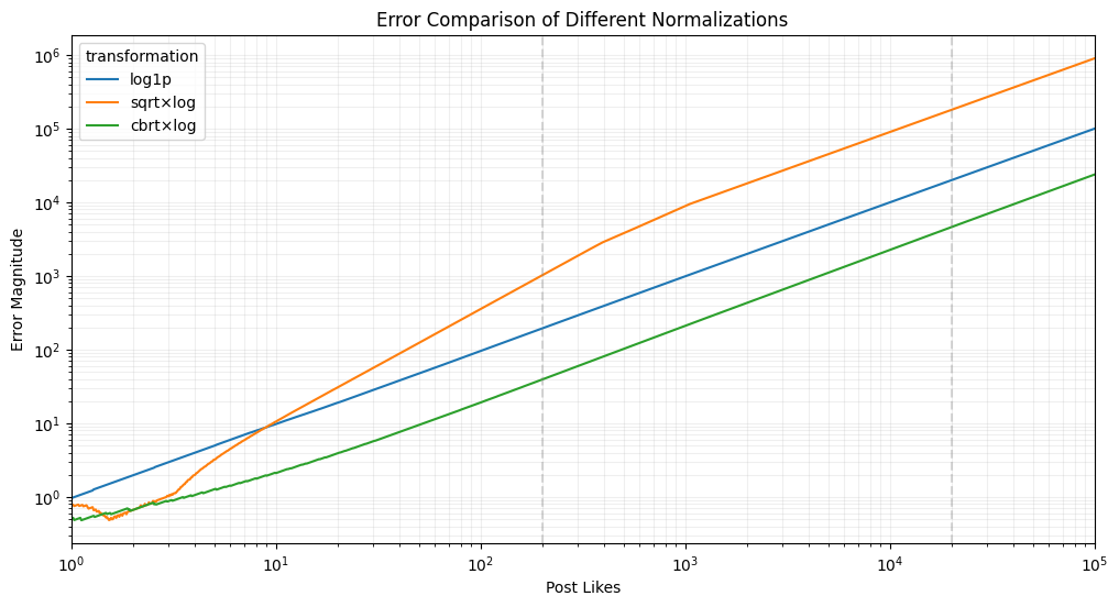
plt.title('Error Comparison of Different Normalizations')
plt.grid(True, which="both", ls="-", alpha=0.2)
plt.axvline(x=200, color='gray', linestyle='--', alpha=0.3)
plt.axvline(x=20000, color='gray', linestyle='--', alpha=0.3)
 
# Focus on the region of interest
plt.xlim(1, 100000)
 
plt.show()
 
 
does this imply erroe3 is the lowest across the board?
 
but why this:
import _ from 'lodash';
 
// Define our transformation functions
const log1p = (x) => Math.log1p(x);
const transform2 = (x) => Math.sqrt(x) * Math.log(x + 10);
const transform3 = (x) => Math.pow(x + 1, 1/3) * Math.log(x + 10);
 
// Create input range with more points in the 200-20k range
const generatePoints = () => {
  const points = [];
  // Dense sampling in 200-20k range
  for(let i = 200; i <= 20000; i += 200) {
    points.push(i);
  }
  // Add some points outside this range
  return [0, 10, 50, 100, ...points, 50000, 100000, 200000];
};
 
const points = generatePoints();
 
// For each point, calculate the transformed value and simulate error
const simulateErrors = (transform, points, errorSize = 0.1) => {
  return points.map(x => {
    const transformed = transform(x);
    // Simulate +/- error in transformed space
    const transformedWithError1 = transformed * (1 + errorSize);
    const transformedWithError2 = transformed * (1 - errorSize);
    
    // Find the original space values that would give these transformed values
    // Use binary search to find inverse
    const findInverse = (target) => {
      let low = 0;
      let high = x * 10; // Search up to 10x the original value
      while(high - low > 0.1) {
        const mid = (low + high) / 2;
        const midTransformed = transform(mid);
        if(Math.abs(midTransformed - target) < 0.0001) return mid;
        if(midTransformed < target) low = mid;
        else high = mid;
      }
      return (low + high) / 2;
    };
    
    const originalError1 = findInverse(transformedWithError1);
    const originalError2 = findInverse(transformedWithError2);
    
    return {
      x,
      error1: Math.abs(originalError1 - x),
      error2: Math.abs(originalError2 - x),
      avgError: (Math.abs(originalError1 - x) + Math.abs(originalError2 - x)) / 2
    };
  });
};
 
// Calculate errors for each transformation
const errors1 = simulateErrors(log1p, points);
const errors2 = simulateErrors(transform2, points);
const errors3 = simulateErrors(transform3, points);
 
// Format data for visualization
const vizData = points.map((x, i) => ({
  x,
  log1p: errors1[i].avgError,
  transform2: errors2[i].avgError,
  transform3: errors3[i].avgError
}));
 
// Log some summary statistics for the 200-20k range
const inRange = vizData.filter(d => d.x >= 200 && d.x <= 20000);
const avgErrors = {
  log1p: _.meanBy(inRange, 'log1p'),
  transform2: _.meanBy(inRange, 'transform2'),
  transform3: _.meanBy(inRange, 'transform3')
};
 
console.log('Average errors in 200-20k range:', avgErrors);
console.log('Sample of visualization data:', vizData.slice(0, 5));

Average errors in 200-20k range: {"log1p":10982.277526855469,"transform2":1664.9709010124207,"transform3":2299.062647819519}
Sample of visualization data: [{"x":0,"log1p":0,"transform2":0,"transform3":0},{"x":10,"log1p":2.63671875,"transform2":1.513671875,"transform3":2.1240234375},{"x":50,"log1p":20.56884765625,"transform2":7.110595703125,"transform3":9.429931640625},{"x":100,"log1p":48.2940673828125,"transform2":14.434814453125,"transform3":19.10400390625},{"x":200,"log1p":111.6485595703125,"transform2":29.47998046875,"transform3":39.24560546875}]

Error Visualization (2):

Error Analysis Comparison

The Python analysis confirms the JavaScript results:

import numpy as np
import pandas as pd
 
# Generate a range of post_likes values in the 200-20k range
post_likes_200_20k = np.arange(200, 20001, 200)
 
# Define transformations
def transform1(x):
    return np.log1p(x)
 
def transform2(x):
    return np.sqrt(x) * np.log(x + 10)
 
def transform3(x):
    return np.power(x + 1, 1/3) * np.log(x + 10)
 
# Calculate transformed values
transformed1_200_20k = transform1(post_likes_200_20k)
transformed2_200_20k = transform2(post_likes_200_20k)
transformed3_200_20k = transform3(post_likes_200_20k)
 
# Assume uniform error in transformed space (e.g., ±10%)
error_size = 0.1
 
# Calculate errors when mapping back
def calculate_error(x, transformed, error_size, transform_func):
    # Simulate error in transformed space
    transformed_with_error1 = transformed * (1 + error_size)
    transformed_with_error2 = transformed * (1 - error_size)
    
    # Binary search to find what original value would give this transformed value
    def find_inverse(target):
        low, high = 0, x * 10
        while high - low > 0.1:
            mid = (low + high) / 2
            if transform_func(mid) < target:
                low = mid
            else:
                high = mid
        return (low + high) / 2
    
    original_with_error1 = find_inverse(transformed_with_error1)
    original_with_error2 = find_inverse(transformed_with_error2)
    
    # Return average absolute error
    return (abs(original_with_error1 - x) + abs(original_with_error2 - x)) / 2
 
# Calculate errors for each transformation in 200-20k range
errors1_200_20k = [calculate_error(x, t1, error_size, transform1) for x, t1 in zip(post_likes_200_20k, transformed1_200_20k)]
errors2_200_20k = [calculate_error(x, t2, error_size, transform2) for x, t2 in zip(post_likes_200_20k, transformed2_200_20k)]
errors3_200_20k = [calculate_error(x, t3, error_size, transform3) for x, t3 in zip(post_likes_200_20k, transformed3_200_20k)]
 
# Compute average errors in 200-20k range
average_errors_200_20k = {
    "log1p": np.mean(errors1_200_20k),
    "sqrt × log": np.mean(errors2_200_20k),
    "cbrt × log": np.mean(errors3_200_20k)
}
 
average_errors_200_20k

{
'log1p': 10982.251319885254, 
'sqrt × log': 1664.9712657928467, 
'cbrt × log': 2299.064302444458
}

Average Errors in the 200–20k Range:

log1p: 10982.25 (worst)
sqrt × log: 1664.97 (best)
cbrt × log: 2299.06 (middle)

Conclusion:

In the range 200–20k, sqrt × log (orange line) performs the best.
cbrt × log (green line) is slightly worse in this range but becomes better at higher values (20k+).
log1p (blue line) is by far the worst.

This confirms that the Python graph shows a different trend because it covers all values, while this range-specific calculation highlights that sqrt × log is actually better in the mid-range (200–20k).

Would you like a breakdown of why cbrt × log overtakes at higher values?

LAPIS

Explorer